The Getting started vignette should be read before this one. Here we explain all the grouping functionality supported by casteval.
Group columns
On top of the time, sim, val,
val_mean, etc. columns that can be in forecast data frames,
a forecast data frame can contain as many grouping columns as you like.
A grouping column starts with grp_ followed by a nonempty
string, for example grp_variable,
grp_scenario, grp_province. These columns can
be used to group your forecast data.
# data frame with 3 group columns, each taking on 2 values
# see ?groups1 for details
groups1
#> # A tibble: 16 × 7
#>     time grp_variable grp_province grp_scenario val_q5 val_q95 val_mean
#>    <dbl> <chr>        <chr>               <dbl>  <dbl>   <dbl>    <dbl>
#>  1     1 hosp         ON                      1     10      20       15
#>  2     1 case         ON                      1   1000    2000     1500
#>  3     1 hosp         QC                      1     11      21       16
#>  4     1 case         QC                      1   1100    2100     1600
#>  5     1 hosp         ON                      2     15      25       20
#>  6     1 case         ON                      2   1500    2500     2000
#>  7     1 hosp         QC                      2     16      26       21
#>  8     1 case         QC                      2   1600    2600     2100
#>  9     2 hosp         ON                      1     50      60       55
#> 10     2 case         ON                      1   5000    6000     5500
#> 11     2 hosp         QC                      1     51      61       56
#> 12     2 case         QC                      1   5100    6100     5600
#> 13     2 hosp         ON                      2     55      65       60
#> 14     2 case         ON                      2   5500    6500     6000
#> 15     2 hosp         QC                      2     56      66       61
#> 16     2 case         QC                      2   5600    6600     6100
# a similar data frame but with raw data
groups2
#> # A tibble: 32 × 5
#>     time grp_variable grp_province grp_scenario   val
#>    <dbl> <chr>        <chr>               <dbl> <dbl>
#>  1     1 hosp         ON                      1    15
#>  2     1 hosp         ON                      1    15
#>  3     1 case         ON                      1  1499
#>  4     1 case         ON                      1  1501
#>  5     1 hosp         QC                      1    14
#>  6     1 hosp         QC                      1    18
#>  7     1 case         QC                      1  1597
#>  8     1 case         QC                      1  1603
#>  9     1 hosp         ON                      2    16
#> 10     1 hosp         ON                      2    24
#> # ℹ 22 more rows
Similarly, observations data frames can also contain group columns.
# an observations data frame with the same grouping columns as above
groups_obs
#> # A tibble: 16 × 5
#>     time grp_variable grp_province grp_scenario val_obs
#>    <dbl> <chr>        <chr>               <dbl>   <dbl>
#>  1     1 hosp         ON                      1       9
#>  2     1 case         ON                      1    1000
#>  3     1 hosp         QC                      1      12
#>  4     1 case         QC                      1    1599
#>  5     1 hosp         ON                      2      20
#>  6     1 case         ON                      2    2001
#>  7     1 hosp         QC                      2      24
#>  8     1 case         QC                      2    2500
#>  9     2 hosp         ON                      1      27
#> 10     2 case         ON                      1      10
#> 11     2 hosp         QC                      1      11
#> 12     2 case         QC                      1      12
#> 13     2 hosp         ON                      2      13
#> 14     2 case         ON                      2      14
#> 15     2 hosp         QC                      2      15
#> 16     2 case         QC                      2      16
Scoring
Scoring functions behave a little differently when given grouped data. For a forecast and observations to be compatible for scoring, they must have the exact same group columns.1
If summarize=TRUE, then the result will be a data frame
with the usual val_obs and score columns, as
well as the group columns present in the forecast/observations.
fc1 <- create_forecast(groups1)
fc2 <- create_forecast(groups2)

bias(fc2, groups_obs)
#> # A tibble: 8 × 4
#>   grp_variable grp_province grp_scenario score
#>   <chr>        <chr>               <dbl> <dbl>
#> 1 case         ON                      1   1
#> 2 case         ON                      2  -0.5
#> 3 case         QC                      1  -0.5
#> 4 case         QC                      2  -1
#> 5 hosp         ON                      1   1
#> 6 hosp         ON                      2  -0.5
#> 7 hosp         QC                      1   0
#> 8 hosp         QC                      2  -0.5
accuracy(fc1, groups_obs)
#> Scoring accuracy using quantile pairs c(5, 95)
#> # A tibble: 8 × 6
#>    pair grp_variable grp_province grp_scenario     n score
#>   <int> <chr>        <chr>               <dbl> <int> <dbl>
#> 1     1 case         ON                      1     2   0.5
#> 2     1 case         ON                      2     2   0.5
#> 3     1 case         QC                      1     2   0.5
#> 4     1 case         QC                      2     2   0.5
#> 5     1 hosp         ON                      1     2   0
#> 6     1 hosp         ON                      2     2   0.5
#> 7     1 hosp         QC                      1     2   0.5
#> 8     1 hosp         QC                      2     2   0.5
# accuracy still works with multiple quantile pairs
accuracy(fc2, groups_obs, quant_pairs=list(c(5,95), c(25,75)))
#> Scoring accuracy using quantile pairs c(5, 95), c(25, 75)
#> # A tibble: 16 × 6
#>     pair grp_variable grp_province grp_scenario     n score
#>    <int> <chr>        <chr>               <dbl> <int> <dbl>
#>  1     1 case         ON                      1     2   0
#>  2     1 case         ON                      2     2   0.5
#>  3     1 case         QC                      1     2   0.5
#>  4     1 case         QC                      2     2   0
#>  5     1 hosp         ON                      1     2   0
#>  6     1 hosp         ON                      2     2   0.5
#>  7     1 hosp         QC                      1     2   0
#>  8     1 hosp         QC                      2     2   0.5
#>  9     2 case         ON                      1     2   0
#> 10     2 case         ON                      2     2   0.5
#> 11     2 case         QC                      1     2   0.5
#> 12     2 case         QC                      2     2   0
#> 13     2 hosp         ON                      1     2   0
#> 14     2 hosp         ON                      2     2   0.5
#> 15     2 hosp         QC                      1     2   0
#> 16     2 hosp         QC                      2     2   0.5
crps(fc2, groups_obs, at=2)
#> # A tibble: 8 × 4
#>   grp_variable grp_province grp_scenario   score
#>   <chr>        <chr>               <dbl>   <dbl>
#> 1 case         ON                      1 5485
#> 2 case         ON                      2    6.25
#> 3 case         QC                      1    8.25
#> 4 case         QC                      2    4.25
#> 5 hosp         ON                      1   23.5
#> 6 hosp         ON                      2    7.25
#> 7 hosp         QC                      1    9.25
#> 8 hosp         QC                      2    5.25
If summarize=FALSE, the output will be like a regular
unsummarized data frame plus the group columns.
bias(fc2, groups_obs, summarize=FALSE)
#> # A tibble: 16 × 6
#>    grp_variable grp_province grp_scenario  time val_obs score
#>    <chr>        <chr>               <dbl> <dbl>   <dbl> <dbl>
#>  1 case         ON                      1     1    1000     1
#>  2 case         ON                      1     2      10     1
#>  3 case         ON                      2     1    2001     0
#>  4 case         ON                      2     2      14    -1
#>  5 case         QC                      1     1    1599     0
#>  6 case         QC                      1     2      12    -1
#>  7 case         QC                      2     1    2500    -1
#>  8 case         QC                      2     2      16    -1
#>  9 hosp         ON                      1     1       9     1
#> 10 hosp         ON                      1     2      27     1
#> 11 hosp         ON                      2     1      20     0
#> 12 hosp         ON                      2     2      13    -1
#> 13 hosp         QC                      1     1      12     1
#> 14 hosp         QC                      1     2      11    -1
#> 15 hosp         QC                      2     1      24     0
#> 16 hosp         QC                      2     2      15    -1
crps(fc2, groups_obs, summarize=FALSE)
#> # A tibble: 16 × 6
#>     time grp_variable grp_province grp_scenario   score val_obs
#>    <dbl> <chr>        <chr>               <dbl>   <dbl>   <dbl>
#>  1     1 case         ON                      1  500.      1000
#>  2     1 case         ON                      2    2.5     2001
#>  3     1 case         QC                      1    1.5     1599
#>  4     1 case         QC                      2  396       2500
#>  5     1 hosp         ON                      1    6          9
#>  6     1 hosp         ON                      2    2         20
#>  7     1 hosp         QC                      1    3         12
#>  8     1 hosp         QC                      2    3         24
#>  9     2 case         ON                      1 5485         10
#> 10     2 case         ON                      2    6.25      14
#> 11     2 case         QC                      1    8.25      12
#> 12     2 case         QC                      2    4.25      16
#> 13     2 hosp         ON                      1   23.5       27
#> 14     2 hosp         ON                      2    7.25      13
#> 15     2 hosp         QC                      1    9.25      11
#> 16     2 hosp         QC                      2    5.25      15
accuracy(fc2, groups_obs, quant_pairs=list(c(5,95), c(25,75)), summarize=FALSE)
#> Scoring accuracy using quantile pairs c(5, 95), c(25, 75)
#> # A tibble: 32 × 7
#>     time grp_variable grp_province grp_scenario val_obs score  pair
#>    <dbl> <chr>        <chr>               <dbl>   <dbl> <lgl> <int>
#>  1     1 hosp         ON                      1       9 FALSE     1
#>  2     1 case         ON                      1    1000 FALSE     1
#>  3     1 hosp         QC                      1      12 FALSE     1
#>  4     1 case         QC                      1    1599 TRUE      1
#>  5     1 hosp         ON                      2      20 TRUE      1
#>  6     1 case         ON                      2    2001 TRUE      1
#>  7     1 hosp         QC                      2      24 TRUE      1
#>  8     1 case         QC                      2    2500 FALSE     1
#>  9     2 hosp         ON                      1      27 FALSE     1
#> 10     2 case         ON                      1      10 FALSE     1
#> # ℹ 22 more rows
These unsummarized data frames remain compatible with plotting functions, as explained below.
Plotting
Every plotting function2 supports grouping of its inputs (forecasts and observations). However, there are some caveats.
Up to two grouping columns in the input to a plotting function may
take on multiple values. For example,
groups1 |> dplyr::filter(grp_scenario==1) is a valid
plotting input, but groups1 is not, since it has 3 groups
which take on multiple values.
Therefore at the moment, if you want to plot forecasts/observations
with more than 3 groups, you will probably have to use
dplyr::filter() and iteration in order to generate multiple
plots.3
If 1 group column takes on multiple values, then
ggplot2::facet_wrap() will be used.
fc <- create_forecast(groups1 |> dplyr::filter(grp_scenario==1, grp_variable=="hosp"))
obs <- groups_obs |> dplyr::filter(grp_scenario==1, grp_variable=="hosp")

plot_forecast(fc, obs, score=bias)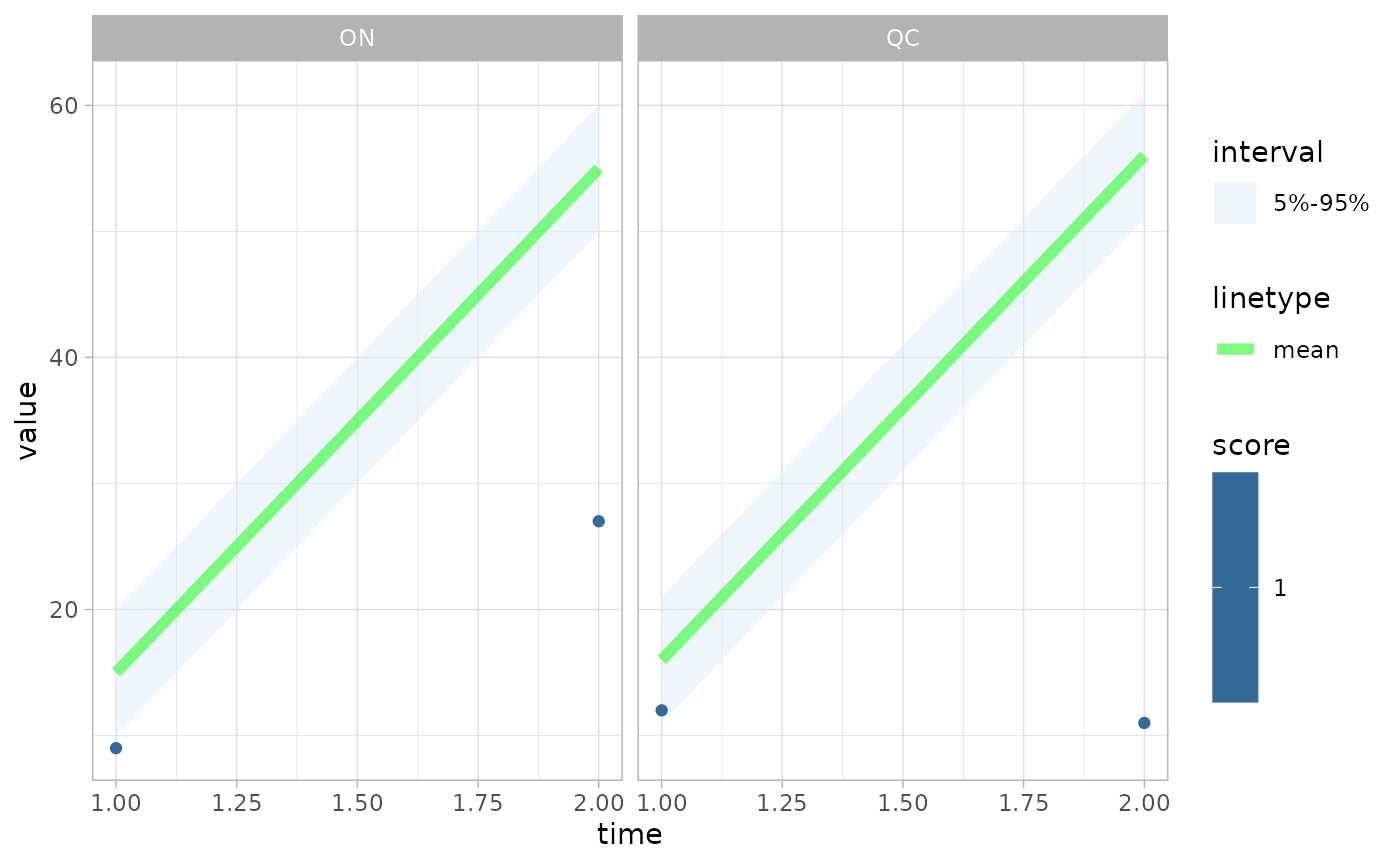
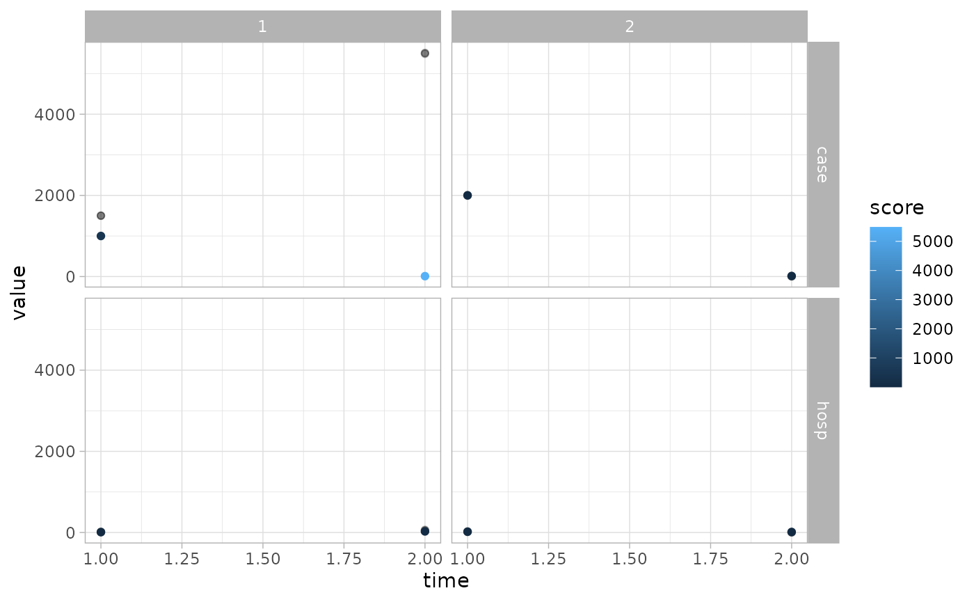
If 2 group columns take on multiple values, then
ggplot2::facet_grid() will be used.
fc <- create_forecast(groups2 |> dplyr::filter(grp_province=="ON"))
obs <- groups_obs |> dplyr::filter(grp_province=="ON")
plot_forecast(fc, obs, score=crps)