Evaluate time series forecasts with casteval • casteval

Overview

casteval is an R package that helps you automate the evaluation of time series forecasts. It provides functionality for formatting, processing, scoring, and visualizing forecasts.

A typical workflow using casteval is:

Create a forecast object by inputting a forecast and its metadata into create_forecast()
Score the forecast using score(), which accepts forecast object(s), corresponding observations, and a particular scoring function
Visualize the forecast using plot_forecast() with a scored forecast and observations

This vignette guides you through this process.

Create a forecast object

In order to create a forecast object, a forecast must first be cast in one of the accepted formats, namely as a data frame or as a list.

Forecast input as data frames

Forecast data frames must contain:

a time column, which can contain either numbers, dates, or date-times
forecast data, which can be passed as raw or summarized.

Raw forecast data are the individual realizations of a model. Summarized forecast data describes an ensemble of realizations by quantiles computed for each time point.

Raw forecast data

Raw forecast data must be passed in a column named val. A sim column may be provided optionally to identify different realizations (enables some scoring and plotting features).

# raw forecast over with numeric times, without simulation numbers
data.frame(
  time=rep(1:5,each=3),
  val=c(
    100, 110, 120, 130, 140,
    101, 111, 121, 131, 141,
    102, 112, 122, 132, 142
  )
)
#>    time val
#> 1     1 100
#> 2     1 110
#> 3     1 120
#> 4     2 130
#> 5     2 140
#> 6     2 101
#> 7     3 111
#> 8     3 121
#> 9     3 131
#> 10    4 141
#> 11    4 102
#> 12    4 112
#> 13    5 122
#> 14    5 132
#> 15    5 142
# raw forecast data with dates, with simulation numbers
data.frame(
  sim=rep(1:3,each=5),
  time=lubridate::as_date(rep(1:5,3)),
  val=c(
    100, 110, 120, 130, 140,
    101, 111, 121, 131, 141,
    102, 112, 122, 132, 142
  )
)
#>    sim       time val
#> 1    1 1970-01-02 100
#> 2    1 1970-01-03 110
#> 3    1 1970-01-04 120
#> 4    1 1970-01-05 130
#> 5    1 1970-01-06 140
#> 6    2 1970-01-02 101
#> 7    2 1970-01-03 111
#> 8    2 1970-01-04 121
#> 9    2 1970-01-05 131
#> 10   2 1970-01-06 141
#> 11   3 1970-01-02 102
#> 12   3 1970-01-03 112
#> 13   3 1970-01-04 122
#> 14   3 1970-01-05 132
#> 15   3 1970-01-06 142

Summarized forecast data

Summarized forecast data may be stored in the following columns:

Quantile columns must start with val_q followed by a number from 0 to 100, e.g., val_50 would be the 50th quantile, i.e., the median
The mean column must be named val_mean

Note that summarized data never contains a sim column.

# summarized forecast data with the 25th, 50th, and 75th percentiles
data.frame(
  time=lubridate::as_datetime(1:5),
  val_q25=c(100,105,103,104,105),
  val_q50=c(201, 210, 205, 201, 200),
  val_q75=c(304, 305, 303, 303, 302)
)
#>                  time val_q25 val_q50 val_q75
#> 1 1970-01-01 00:00:01     100     201     304
#> 2 1970-01-01 00:00:02     105     210     305
#> 3 1970-01-01 00:00:03     103     205     303
#> 4 1970-01-01 00:00:04     104     201     303
#> 5 1970-01-01 00:00:05     105     200     302
# summarized forecast data with the mean, and the 2.5th and 97.5th percentiles
data.frame(
  time=1:5,
  val_q2.5=c(100,103,104,105,102),
  val_mean=c(150,155,160,155,154),
  val_97.5=c(200,200,2204,205,206)
)
#>   time val_q2.5 val_mean val_97.5
#> 1    1      100      150      200
#> 2    2      103      155      200
#> 3    3      104      160     2204
#> 4    4      105      155      205
#> 5    5      102      154      206

All forecast data columns (val, val_*) as well as the sim column must be numeric.

Forecast input as lists

Forecast data frames are straightforward representations forecasts, though they are innefficient for raw forecast data as the time column gets repeated for each realization. If you have particularly long forecasts and/or many realizations, forecast data frames can quickly grow large, which can be slow to work with. Instead, you may wish to represent your forecast as a list.

casteval accepts raw forecast data as a named list with the following entries:

time: a single vector of times as numbers, dates, or date-times
vals: a list of numeric vectors containing the forecasted values, one per realization, where each vector is the same length as time

Since the individual realizations can be inferred from this casting, there is no need to provide additional information to identify individual realizations (as we did with the sim column above) in order to enable related downstream features.

`create_forecast()`

Forecast objects are created with create_forecast(). Its first argument is dat, which is the forecast data in one of the formats described above.

create_forecast() accepts forecast metadata as additional, optional arguments:

name: a label for the forecast. Plotting functions will use name to title the plots they produce.
forecast_time: the time at which the forecast period begins in dat¹. The forecast_time format must match that of the times in the time entry of dat, and can be used in scoring functions to compute scores only after times relative to forecast_time.

# forecast data with 4 time points and an ensemble of 3 simulations
dat1 <- list(
  time=1:4,
  vals=list(
    c(100, 102, 110, 108),
    c(200, 195, 197, 196),
    c(300, 301, 300, 302)
  )
)

fc1 <- create_forecast(dat1, name="forecast 1", forecast_time=3)

# the same data but formatted as a forecast data frame
dat2 <- data.frame(
  time=rep(1:4, each=3),
  sim=rep(1:3, times=4),
  val=c(100, 200, 300, 102, 195, 301, 110, 197, 300, 108, 196, 302)
)

fc2 <- create_forecast(dat2, name="forecast 2", forecast_time=3)

print(fc1)
#> $name
#> [1] "forecast 1"
#> 
#> $forecast_time
#> [1] 3
#> 
#> $data
#>    time sim val
#> 1     1   1 100
#> 2     2   1 102
#> 3     3   1 110
#> 4     4   1 108
#> 5     1   2 200
#> 6     2   2 195
#> 7     3   2 197
#> 8     4   2 196
#> 9     1   3 300
#> 10    2   3 301
#> 11    3   3 300
#> 12    4   3 302
# aside from the order of rows, the resulting forecast data frames are identical
waldo::compare(dplyr::arrange(fc1$data, time), fc2$data)
#> ✔ No differences
# mean-and-quantiles forecast data
dat3 <- data.frame(
  time=1:5,
  val_q2.5=c(100,103,104,105,102),
  val_mean=c(150,155,160,155,154),
  val_q97.5=c(200,200,2204,205,206)
)

# note how we omit `forecast_time`
fc3 <- create_forecast(
  dat3,
  name="forecast 3"
)

print(fc3)
#> $name
#> [1] "forecast 3"
#> 
#> $forecast_time
#> NULL
#> 
#> $data
#>   time val_q2.5 val_mean val_q97.5
#> 1    1      100      150       200
#> 2    2      103      155       200
#> 3    3      104      160      2204
#> 4    4      105      155       205
#> 5    5      102      154       206

create_forecast() returns a forecast object, which is a list with the following fields:

data: a forecast data frame
name: the name of the forecast, if provided
forecast_time: when the forecast was made, if provided

# a forecast object with no optional metadata
list(
  data=data.frame(
    time=1:5,
    val=6:10
  ),
  name=NULL,
  forecast_time=NULL
)
#> $data
#>   time val
#> 1    1   6
#> 2    2   7
#> 3    3   8
#> 4    4   9
#> 5    5  10
#> 
#> $name
#> NULL
#> 
#> $forecast_time
#> NULL
# a forecast object with metadata
list(
  data=data.frame(
    time=lubridate::as_date(1:5),
    val=6:10
  ),
  name="A forecast",
  forecast_time=lubridate::as_date(3)
)
#> $data
#>         time val
#> 1 1970-01-02   6
#> 2 1970-01-03   7
#> 3 1970-01-04   8
#> 4 1970-01-05   9
#> 5 1970-01-06  10
#> 
#> $name
#> [1] "A forecast"
#> 
#> $forecast_time
#> [1] "1970-01-04"

This list could be created by hand, without the help of create_forecast(), but we recommend the latter approach as create_forecast() validates its inputs to avoid issues downstream. For example, it checks that:

forecast_time’s type is consistent with data
quantile values are logically possible (e.g., median values can’t be smaller than the 25th quantiles)
there are no conflicting rows (e.g., there can’t be two rows with the same time reporting different means)

Score a forecast

Forecasts are scored against observations, which must be passed to casteval in a specific format.

Observations data frames

Observations are passed to casteval in a data frame with a time column and a val_obs column. Similar to forecast data frames, time may be either numeric, dates, or date-times. val_obs must be numeric.

# An observations data frame
data.frame(
  time=1:5,
  val_obs=c(50,60,55,57,59)
)
#>   time val_obs
#> 1    1      50
#> 2    2      60
#> 3    3      55
#> 4    4      57
#> 5    5      59

Scoring functions

We score a forecast using score(), which has the following parameters:

fcsts is either a forecast object or a list of forecast objects
obs is an observations data frame
fun is a scoring function
... are additional parameters which will be passed to fun

Scoring functions which can be passed to score() include:

accuracy(), which calculates the success rate of a forecast’s quantile range predictions
crps(), which calculates the Continuous Ranked Probability Score (CRPS) of a forecast
log_score(), which calculates the (positive) logarithmic score of a forecast
bias(), which calculates how much a forecast overpredicts/underpredicts values

score() scores every forecast passed to it against obs, and returns a score for each one.²

Below are examples of scoring. For a detailed explanation of how scoring works, see the scoring vignette

Visualize forecast evaluation

casteval provides plotting functions which allow you to visualize your forecasts, observations, and sometimes scores. Several modular functions (plot_ensemble(), plot_observations(), etc.) implement individual plotting functionality, while the more user-friendly plot_forecast() combines them all. We describe these functions below.

Plot a forecast

plot_forecast() plots a forecast and optionally overlays observations and quantile intervals, scores the forecast, and color-codes the observations based on score.

For raw forecast data, the quant_intervals parameter is like the quant_pairs parameter in accuracy(), and it is used to draw quantile intervals on the plot.³

If val_q50 is present in the forecast data, then the median will be plotted. Similarly, if val_mean is present, the mean will be plotted.

# Create a forecast
fc <- create_forecast(list(
  time=1:10,
  vals=list(
    c(1,2,3,5,4,5,4,6,6,5),
    c(1,3,5,4,6,5,7,9,8,8),
    c(1,4,3,4,5,6,5,3,2,2),
    c(1,2,4,5,7,8,7,9,10,9)
  )
  ),
  name = "Forecast date: 2024-07-30"
)

# Plot it
plot_forecast(fc)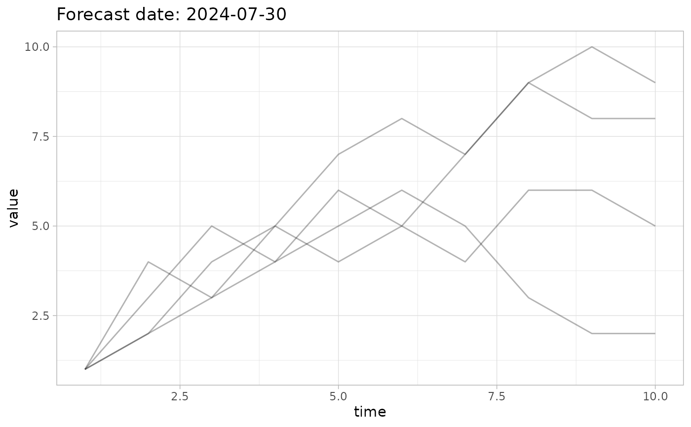

# Plot it and display 3 quantile intervals
plot_forecast(fc, quant_intervals=list(c(25,75), c(2.5,97.5), c(5,95)))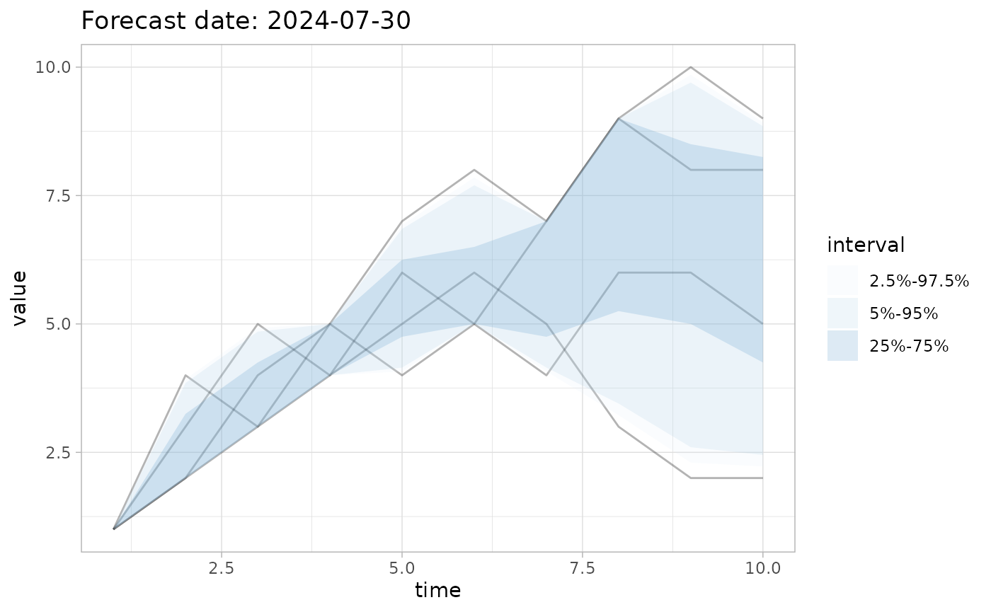

For summarized forecast data, if val_q50 is present in the forecast data, then the median will be plotted. Similarly, if val_mean is present, the mean will be plotted.

# Create a forecast with mean and median data
fc2 <- create_forecast(data.frame(
  time=1:5,
  val_mean=6:10,
  val_q50=c(5.5,6,7.5,9,10)
))

# Plot it
plot_forecast(fc2)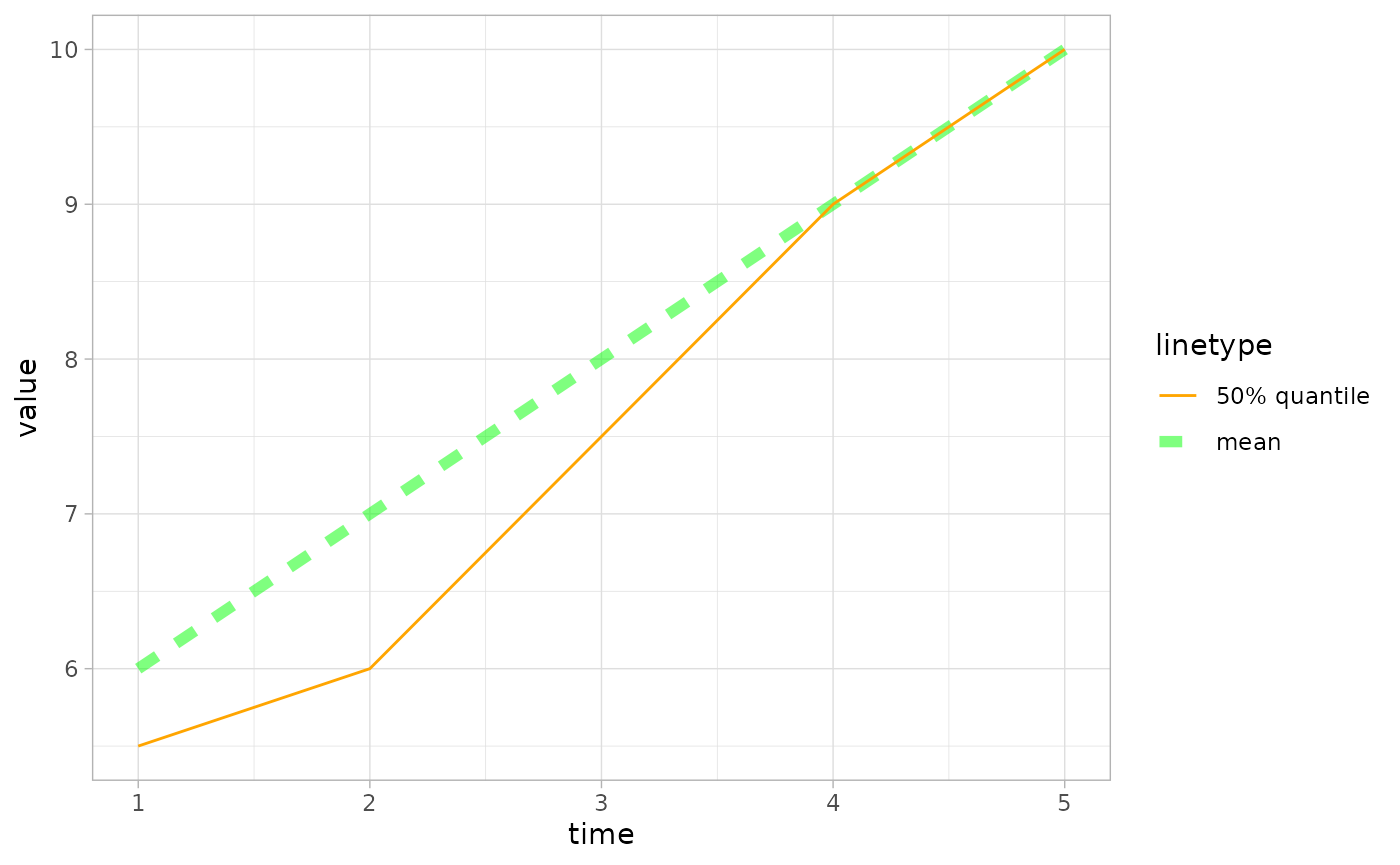

Plot observations with scores

If plot_forecast() is given observations and a scoring function, it can additionally compute scores internally. Just pass a scoring function to the score argument and plot_forecast() will run score(fcst, obs, summarize=FALSE) in order to plot the forecast with observations colour-coded with the scores.

# Create some observations
obs <- data.frame(time=1:10, val_obs=c(1,4,8,10,11,8,5,3,3,2))

# Plot them over the forecast and its quantile intervals
plot_forecast(fc, obs=obs, quant_intervals=list(c(25,75), c(2.5,97.5), c(5,95)))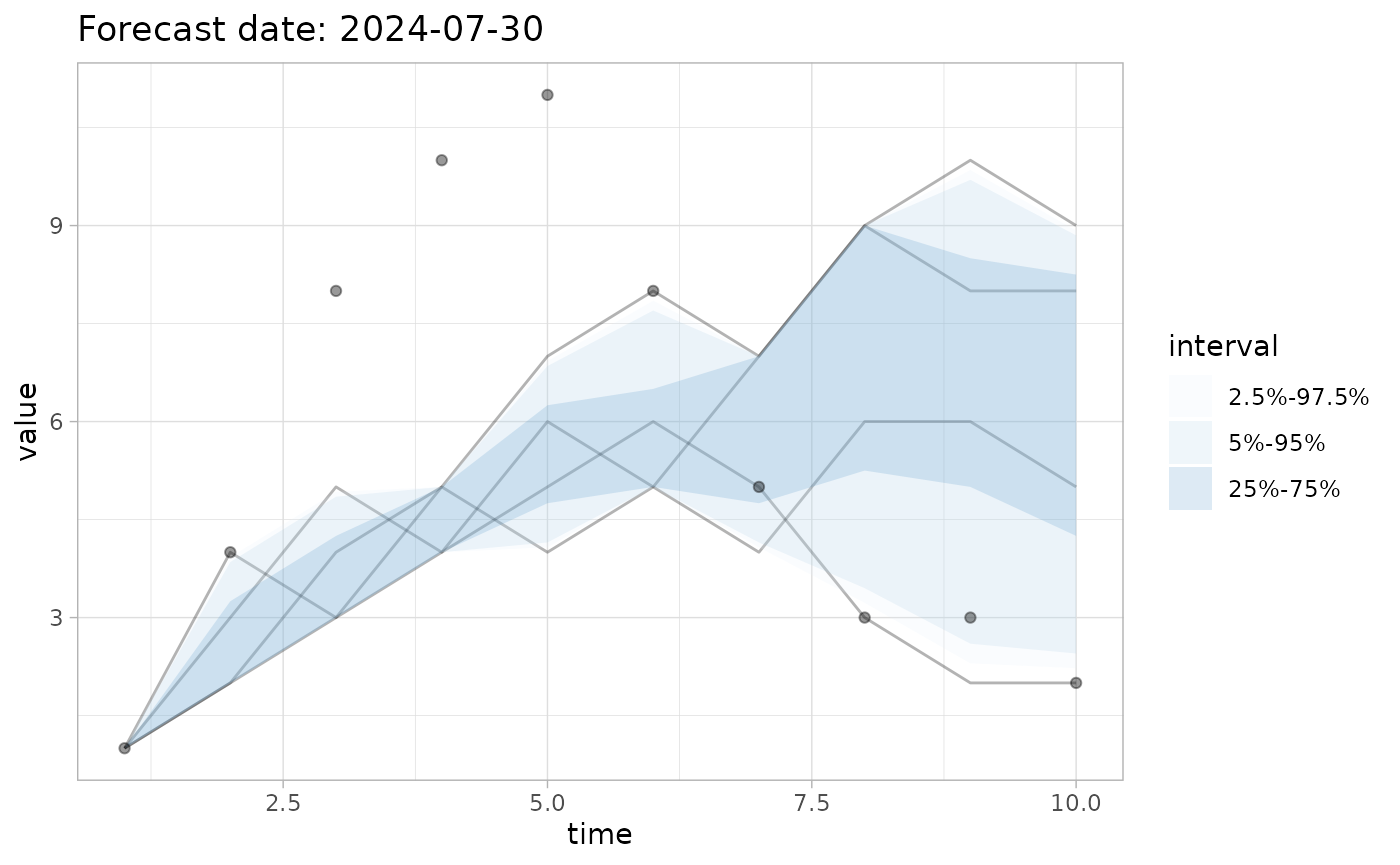

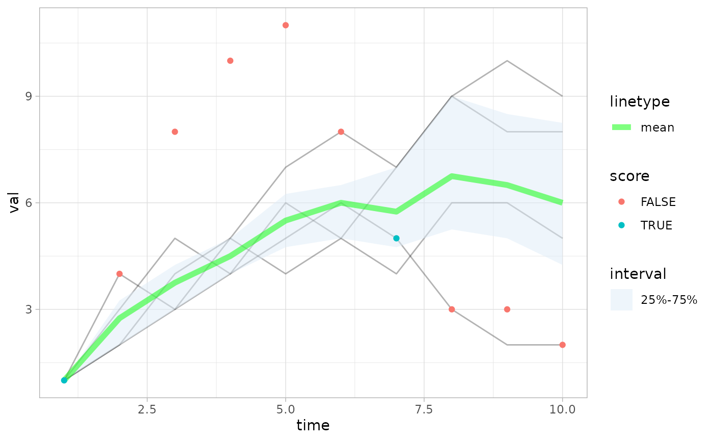
# Colour code points using `log_score()`
# `plot_forecast()` automatically passes `summarize=FALSE` to
# scoring functions in order to obtain the score for each day
plot_forecast(fc, obs=obs, score=log_score, quant_intervals = c(2.5, 97.5))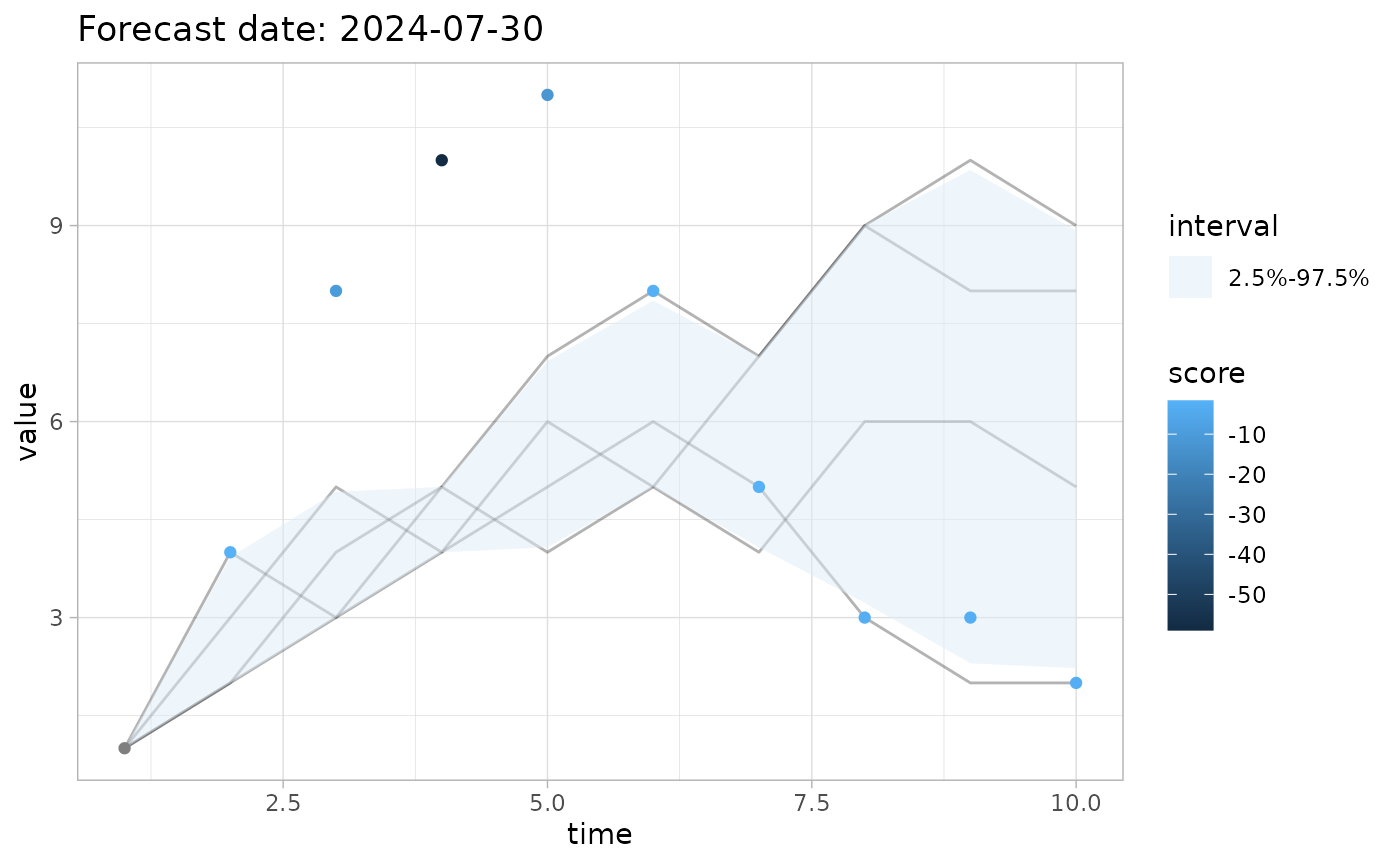

You can pass additional arguments to score through the ellipsis parameter in plot_forecast(). For example, you can specify quantile pairs to accuracy() using this method.

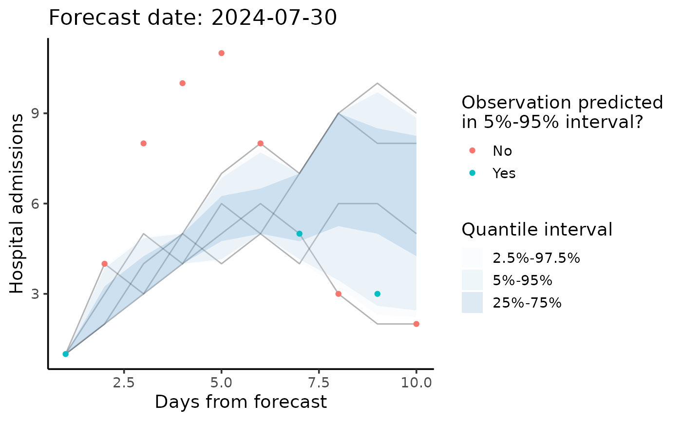
# Identify the observations inside the 5%-95% quantile interval
quant <- c(5,95)
pp <- plot_forecast(fc, obs=obs, quant_intervals=list(c(25,75), c(2.5,97.5), c(5,95)), score=accuracy, quant_pairs=quant)
#> Scoring accuracy using quantile pairs c(5, 95)
pp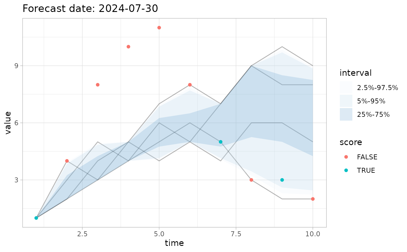

The invert_scale parameter allows you to invert the color scale for observations. For example, for Continuous Ranked Probability Score, a lower score is better.

# don't invert the scale (default behaviour)
plot_forecast(fc, obs, score=crps, invert_scale=FALSE)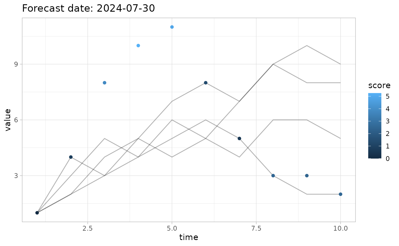

# invert the scale
plot_forecast(fc, obs, score=crps, invert_scale=TRUE)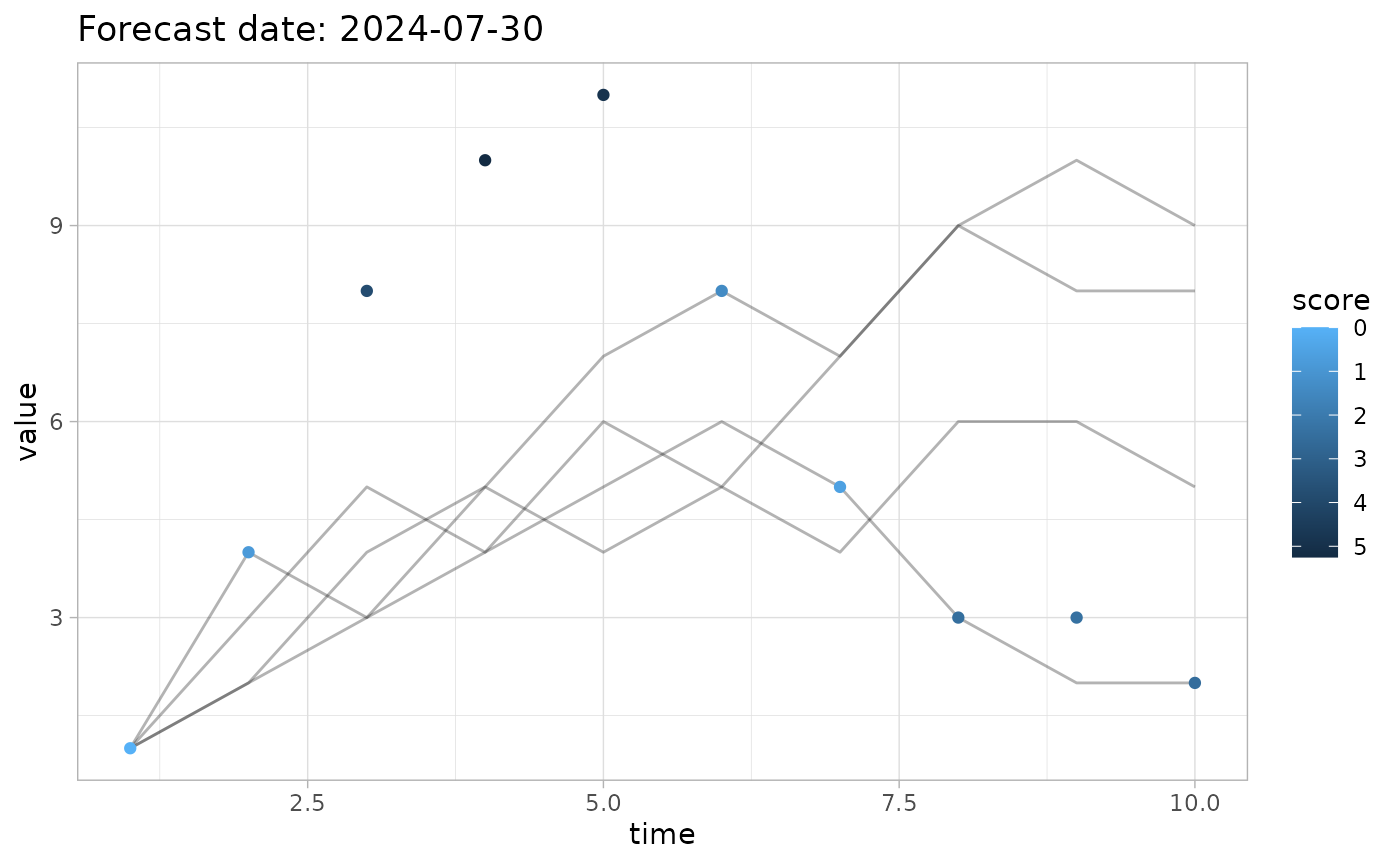

Customize the output

Since plot_forecast() returns a ggplot2::ggplot object, you can further customize the plot to suit your application:

(pp
  + ggplot2::labs(
    x = "Days from forecast",
    y = "Hospital admissions",
    colour = glue::glue("Observation predicted\nin {quant[1]}%-{quant[2]}% interval?"),
    fill = "Quantile interval"  
  )
  + ggplot2::scale_colour_discrete(labels=c(`FALSE`="No", `TRUE`="Yes"))
  + ggplot2::theme_classic(base_size=14)
)

Atomic plotting functions

Behind the scenes, plot_forecast() weaves together the outputs of several helper functions to plot the different aspects of a forecast. If you want further control over the visualization process, you can use these functions directly. They are as follows:

plot_ensemble()⁴ plots an ensemble of forecast realizations⁵
plot_observations() plots a set of observations. If those observations contain a score column, then the scores will be used to colour-code the observations
plot_quantiles() plots the specified quantiles of a forecast (quantiles can also be inferred from the forecast’s data columns).
plot_mean() plots the mean of the forecast data
plot_quant_intervals() uses ggplot2::geom_ribbon() to plot bands of quantile intervals
plot_obs_score() is a wrapper for plot_observations() which allows you to pass a scoring function, scoring parameters, and a forecast to be scored

All these functions consume a ggplot2::ggplot object as their first parameter, and return a ggplot2::ggplot object as well. This makes it possible to compose these functions in any order using a pipe to produce the plot you want.

(plot_ensemble(fcst = fc) 
  |> plot_quant_intervals(fc, c(25,75)) 
  |> plot_mean(fc) 
  |> plot_obs_score(fc, obs, score=accuracy, quant_pairs=c(25,75))
)
#> Scoring accuracy using quantile pairs c(25, 75)